Turbidity Visualization – alternative design

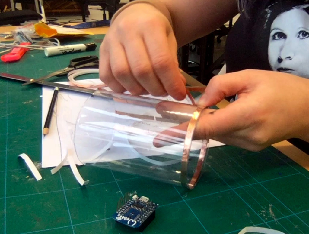
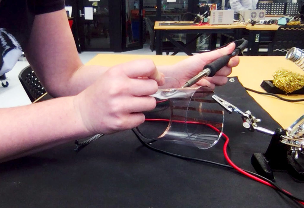
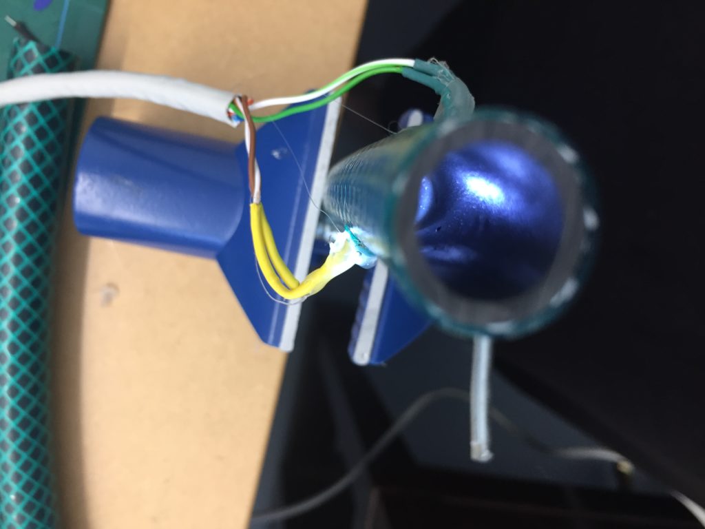
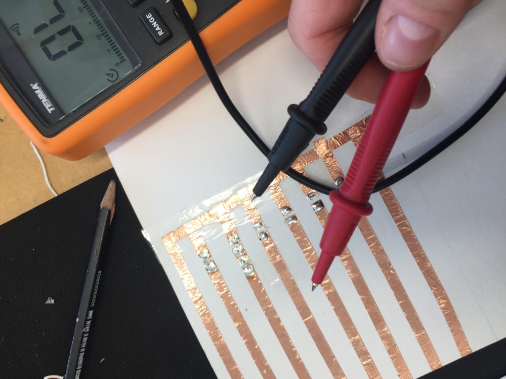
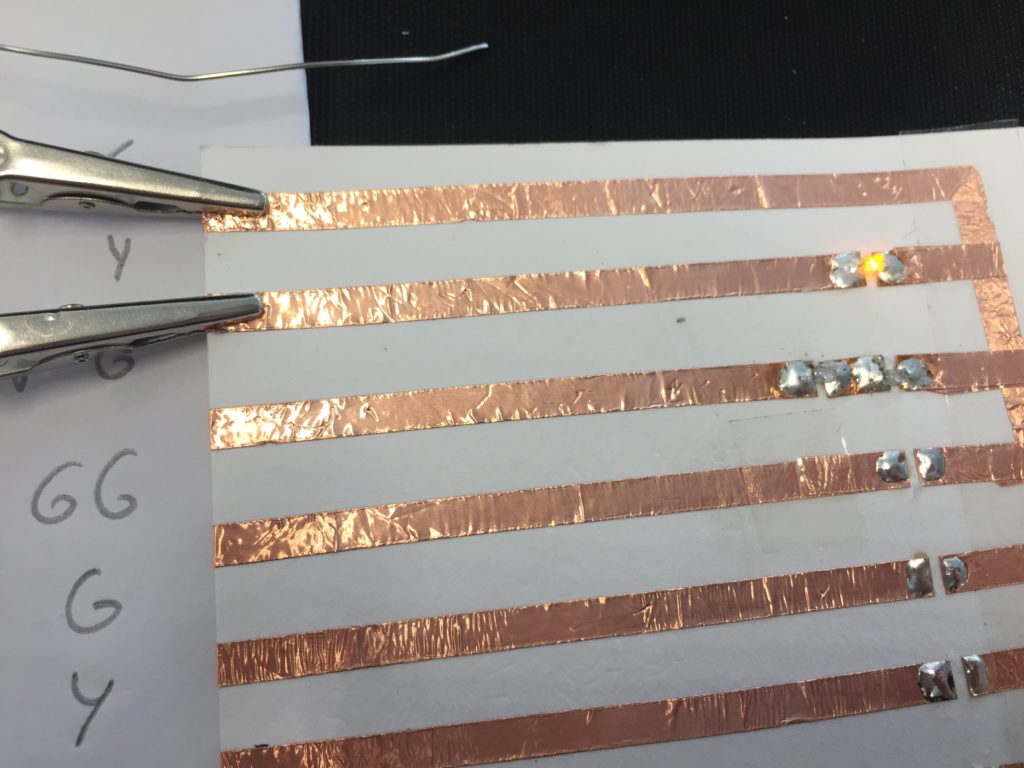
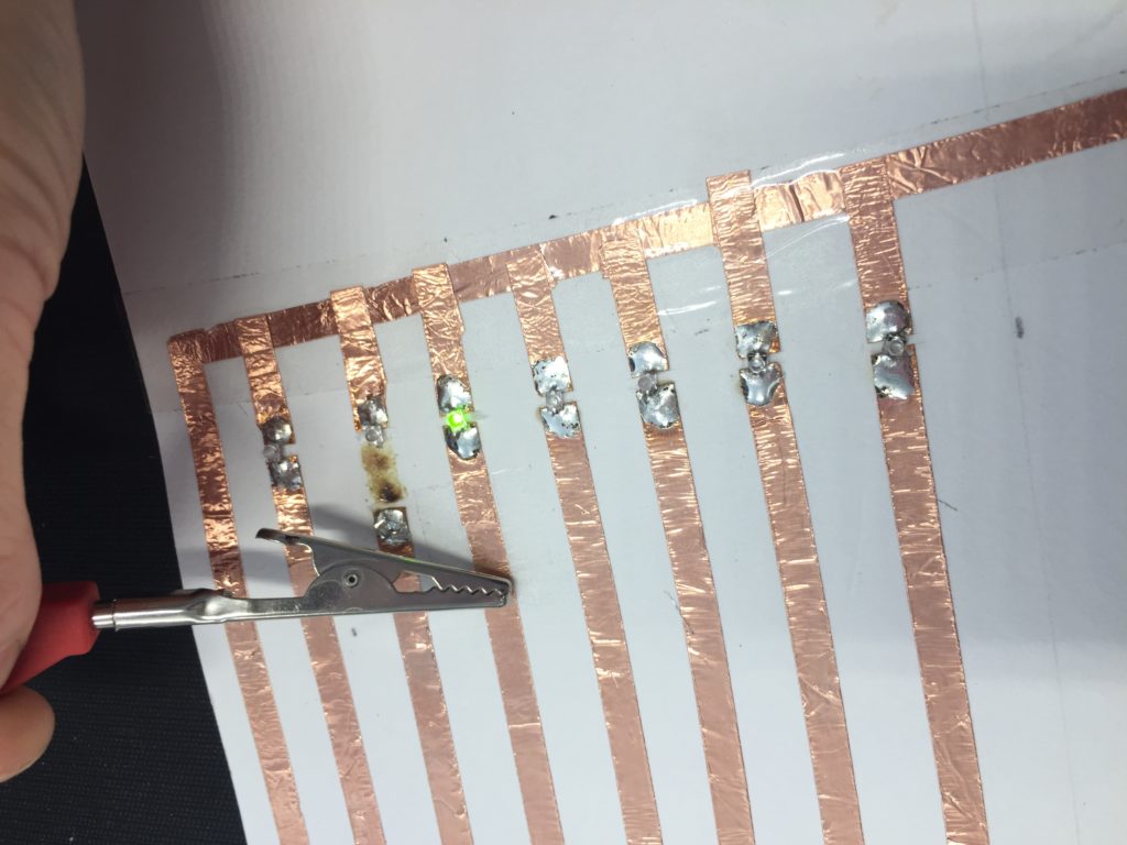
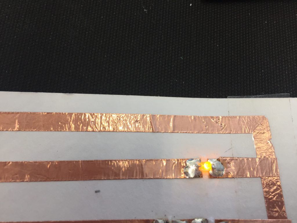
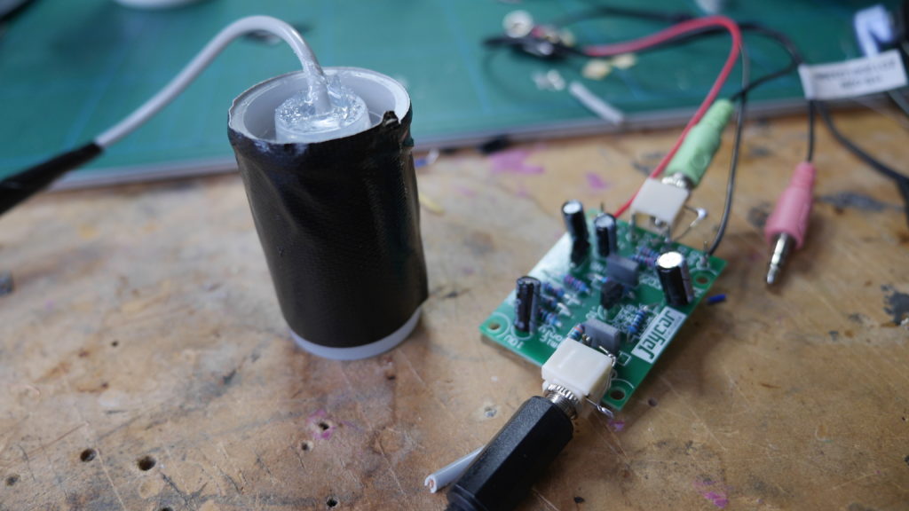
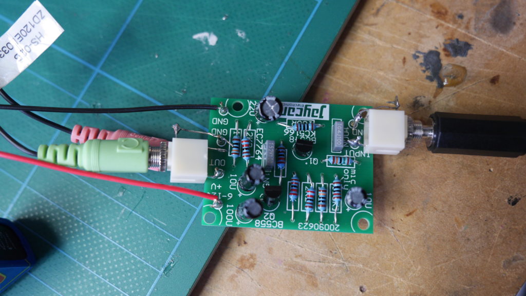
In the first turbidity node design I re-used leftover plastic of one of the bottle designs as the circuit carrier and copper tape for connections. This proved to be tricky as the heat during soldering would distort the plastic and dissolve the glue of the copper tape, making it lift off the surface and weaken the connections.

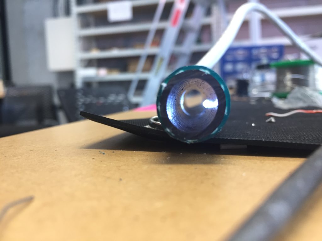
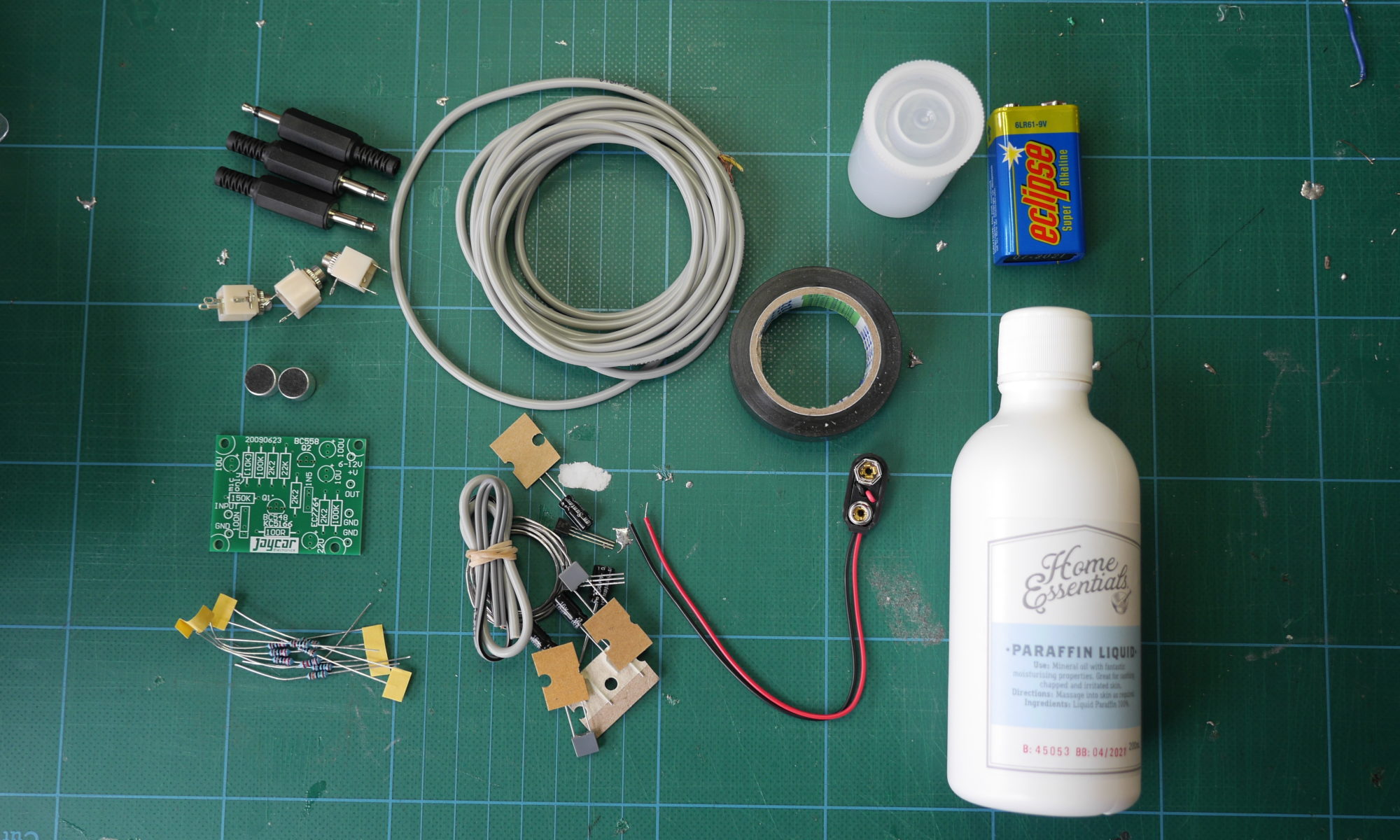
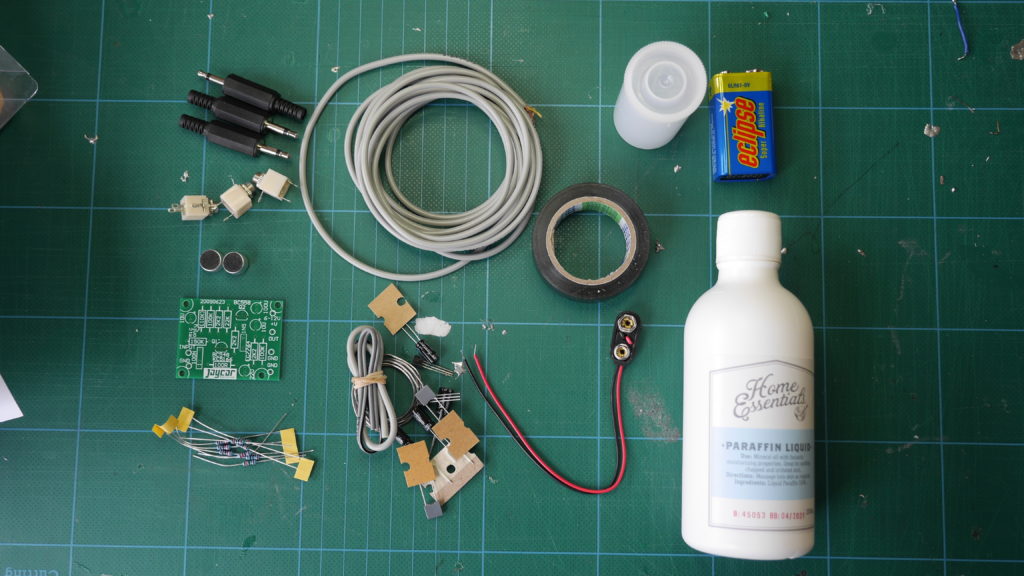
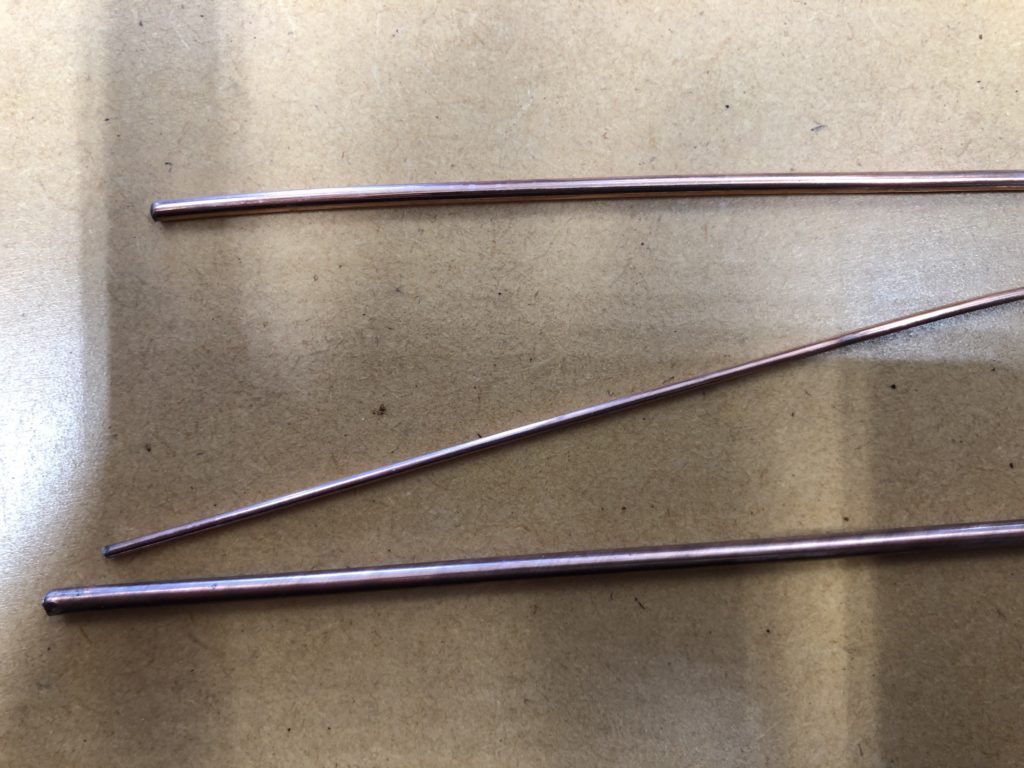
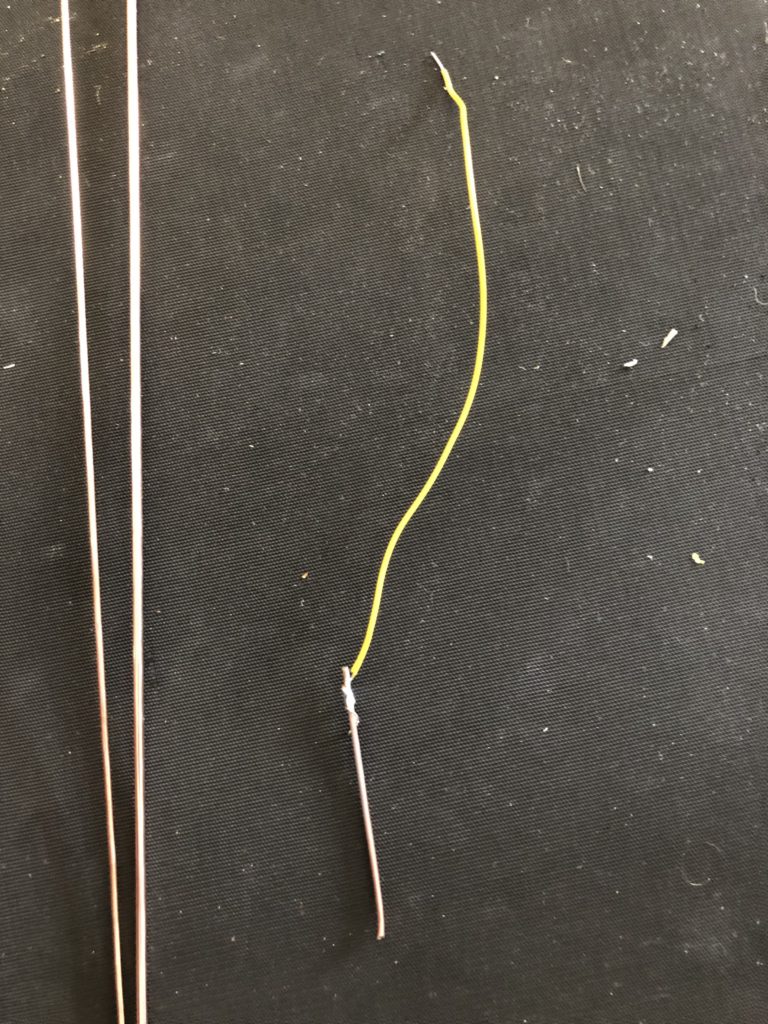
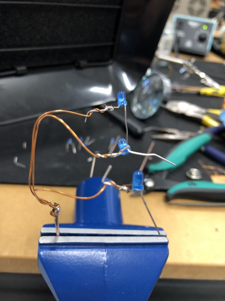
In a new attempt to provide a seamful design, this new prototype uses copper coated welding rods and copper wire as conducting elements and at the same time as structural element. This means the circuit would not require a surface, such as paper or plastic, but would only consist of conducting copper elements. For a first test I used a 1.2mm rod and experimented with soldering various wires and components to the rod. Soldering wire to the copper rod works well after removing the oxidation layer with sandpaper. The enameled copper wire also only solders well after sanding, which is time consuming when many components are involved. The advantage of this, however, is that the 3 dimensional circuit is less likely to be short-circuited, if parts accidentally touch – except for the conductive elements of the LEDs and the solder points.

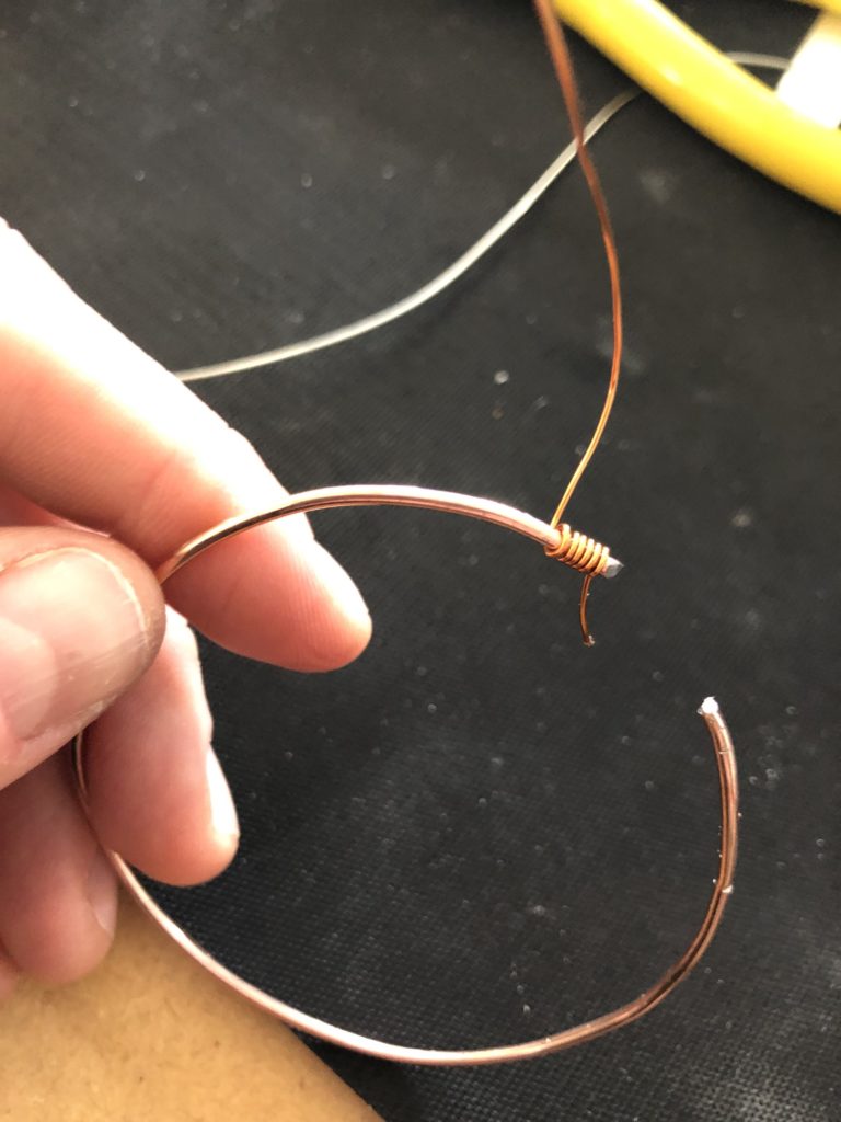
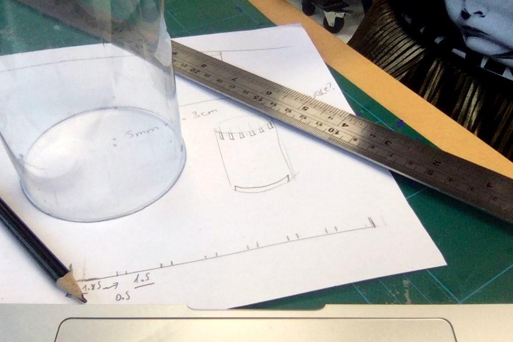
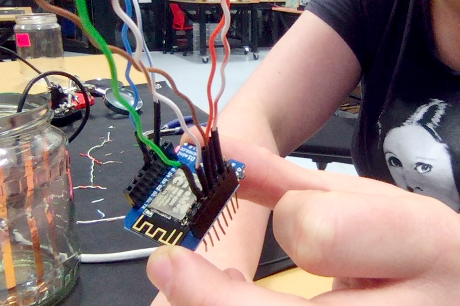
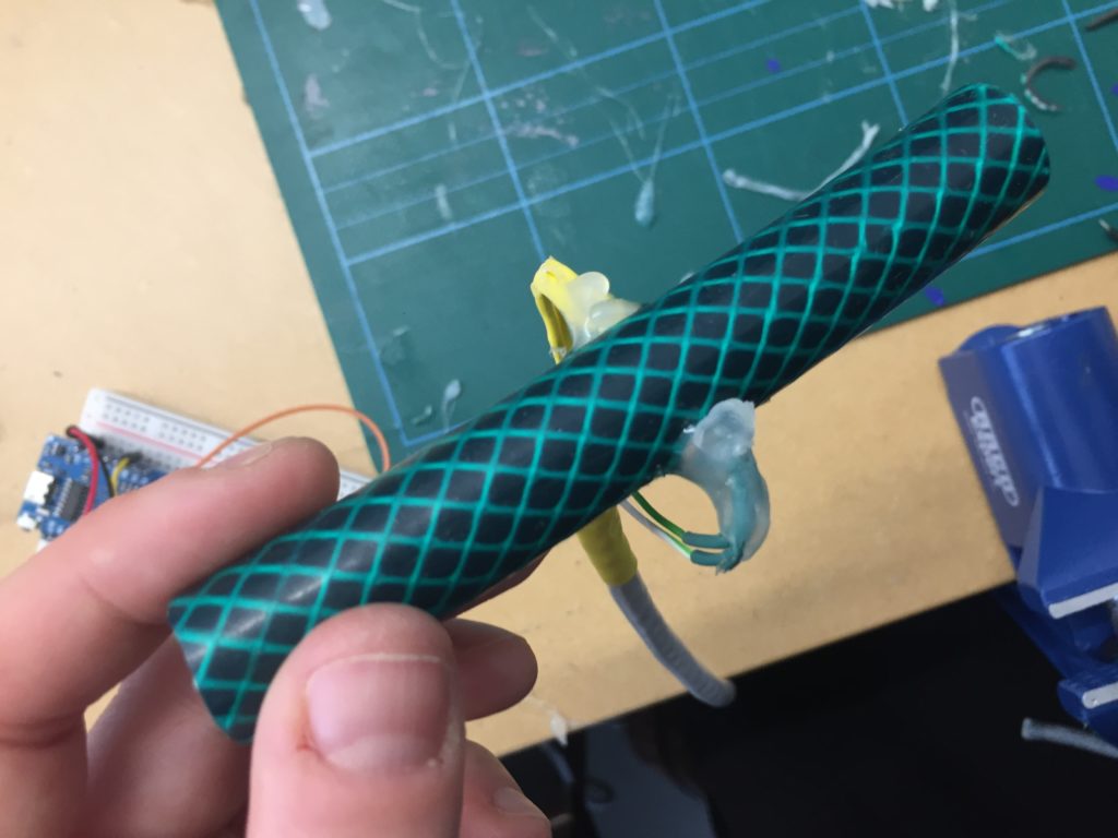
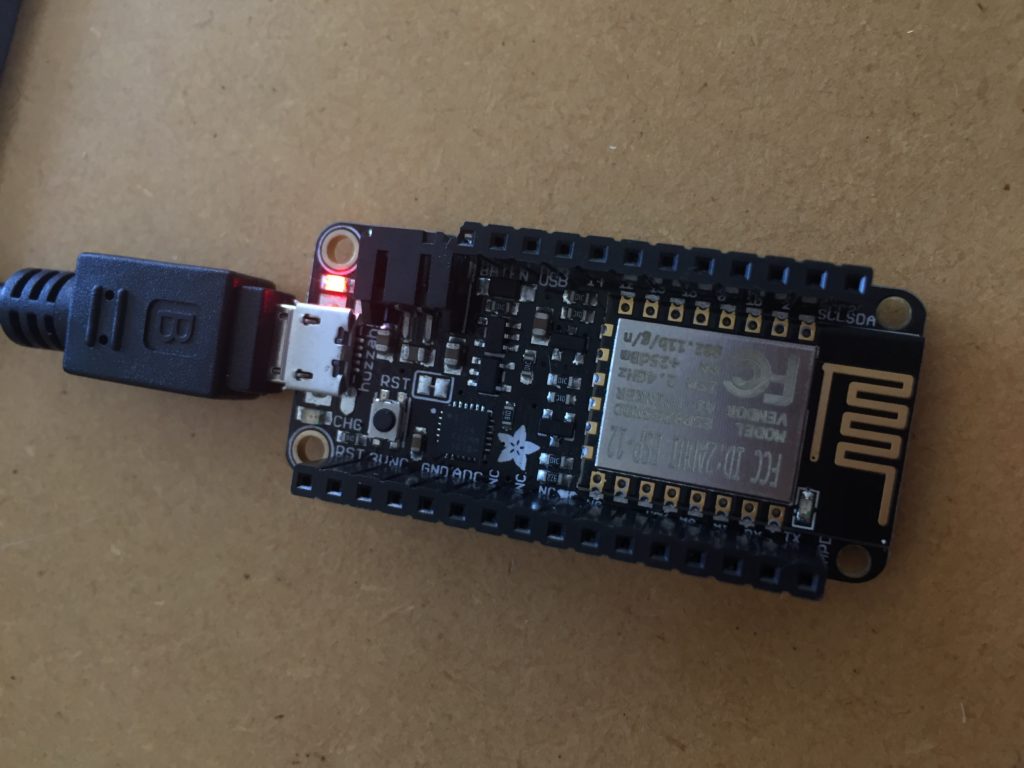
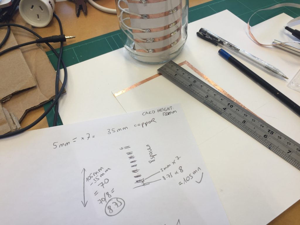
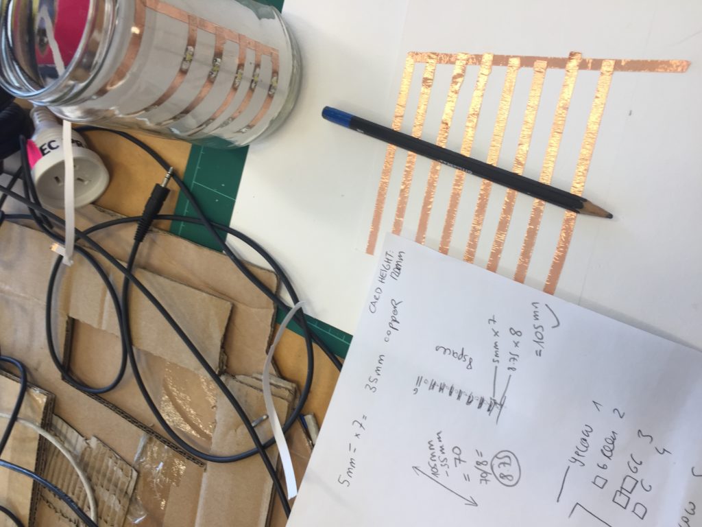
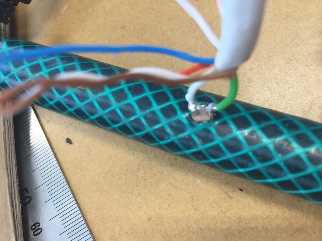
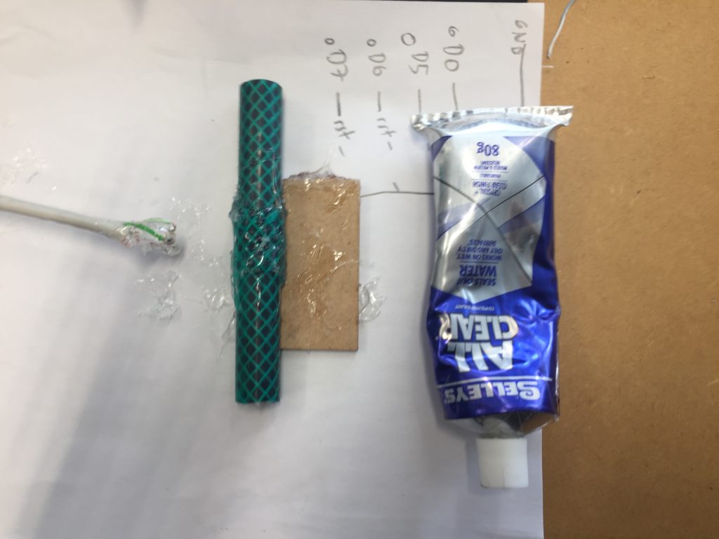
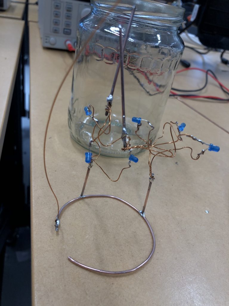
I envisioned the test design to contain a set of 3 addressable LED sets that fit inside a glass jar. I bent the Ground wire into a circular shape to act as a base for the circuit which will connect to a set of LEDs to be controlled by a Wemos D1 board. After a hopeless attempt to use SMD LEDs for this circuit I found that 3mm LED diodes are much better suited for this kind of circuit.

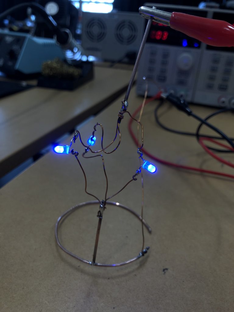
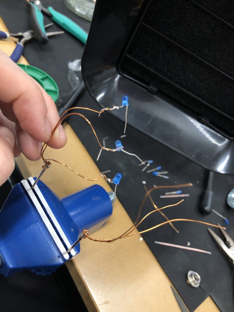
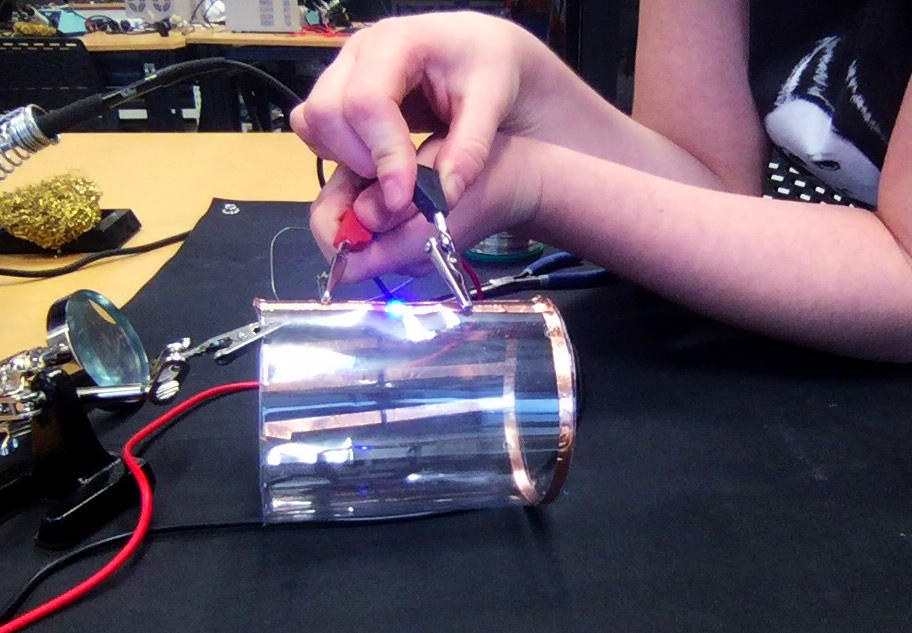
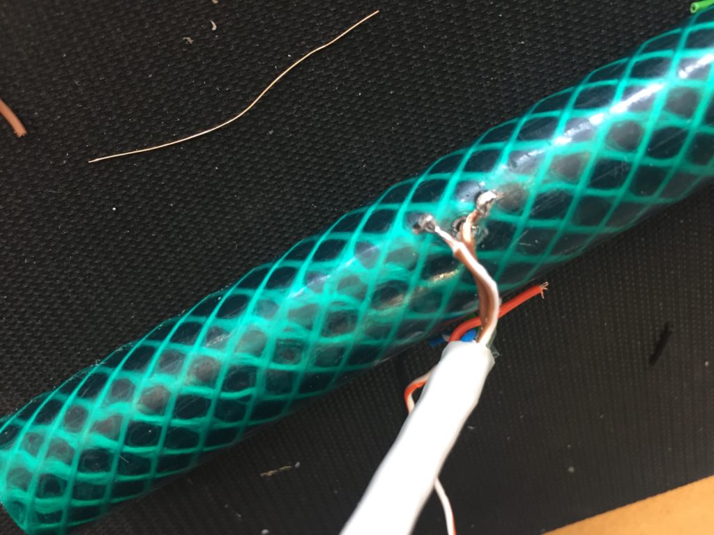
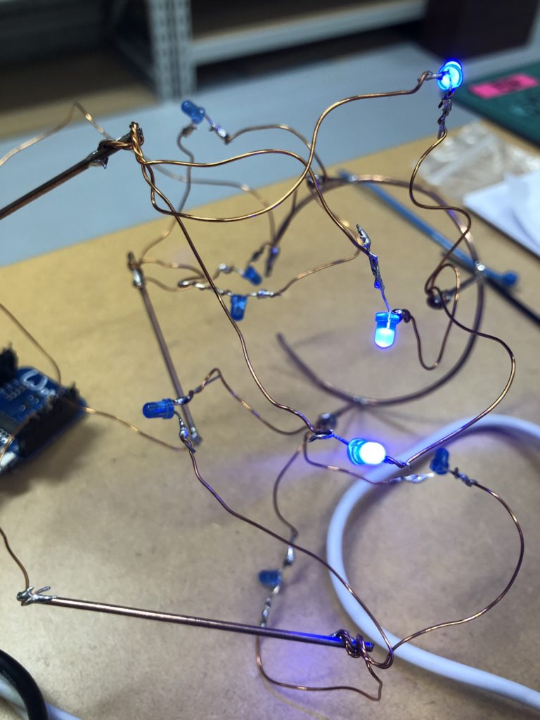
In the end, I connected a set of three LEDs to three individually addressable wires. The copper rod needs to be bent carefully with flat pliers while the copper wire bends into shapes very easily. This gives the final circuit a quite messy look and I am unsure the design in this form would be suitable to provide any meaningful visualization of the turbidity reading.

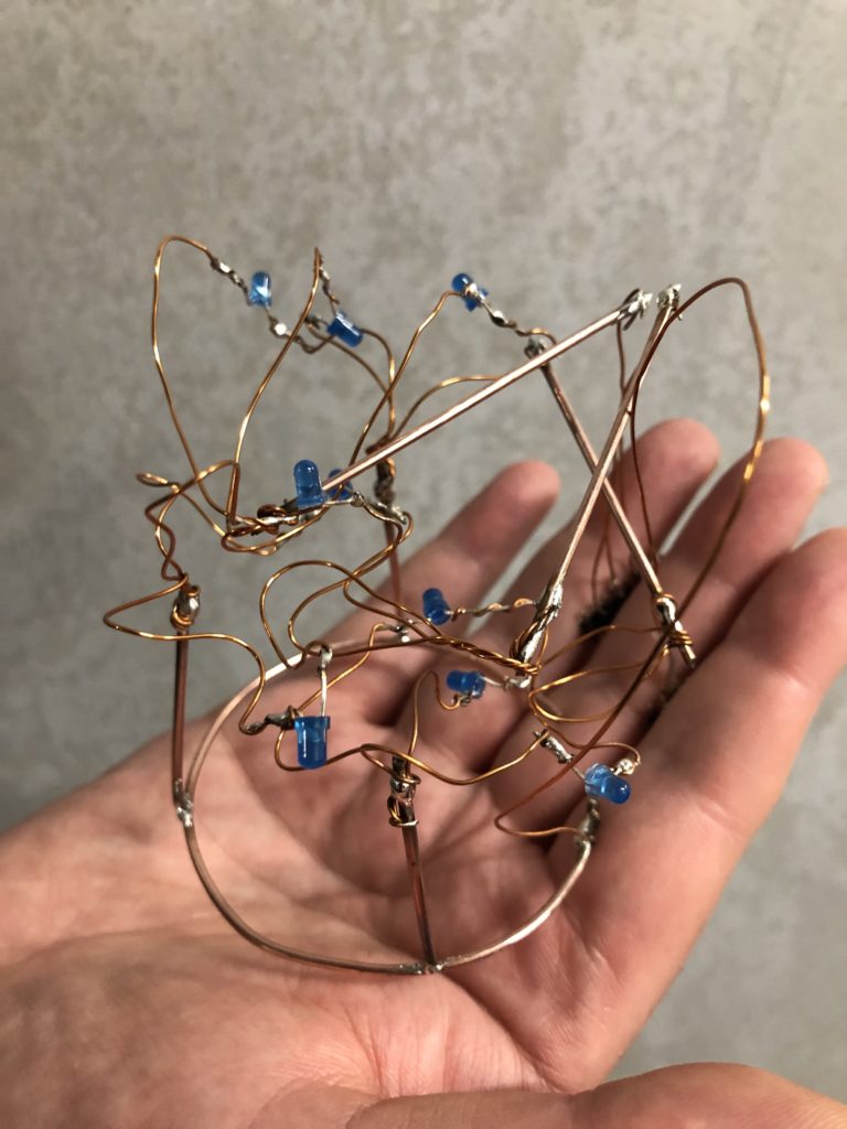
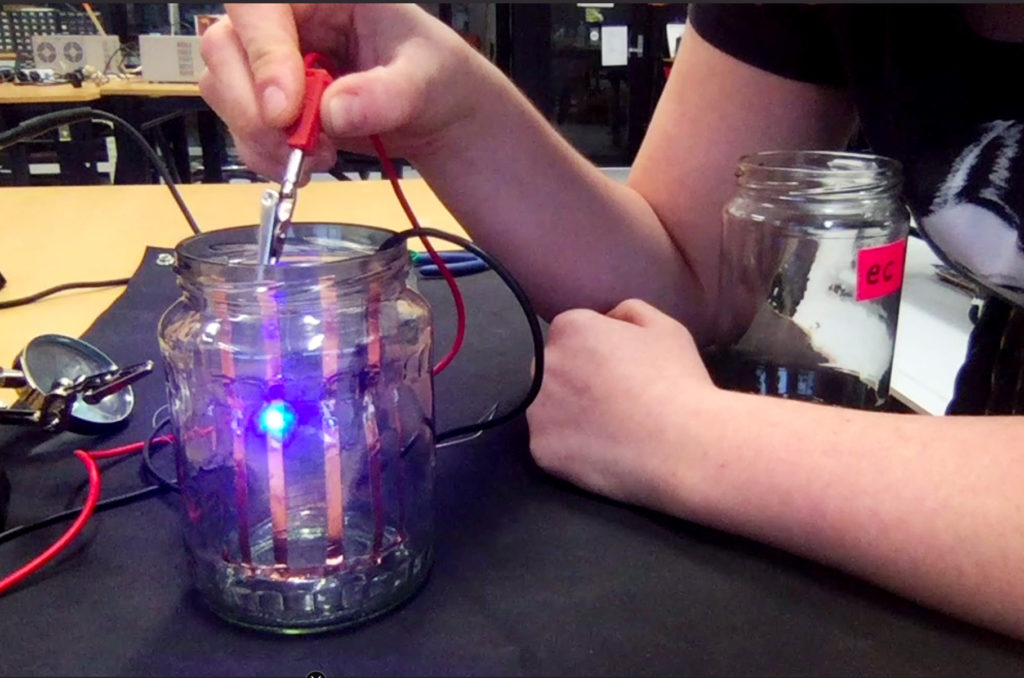
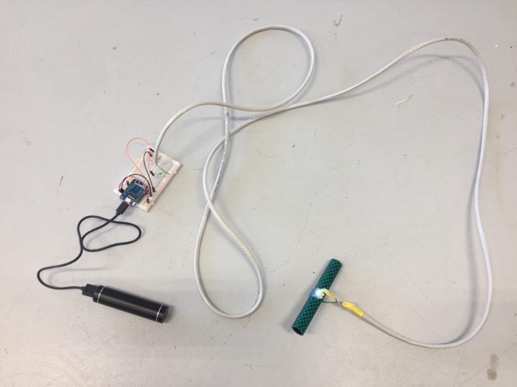
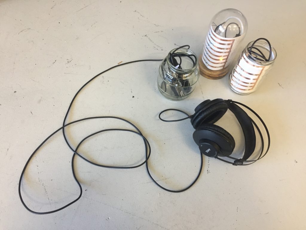
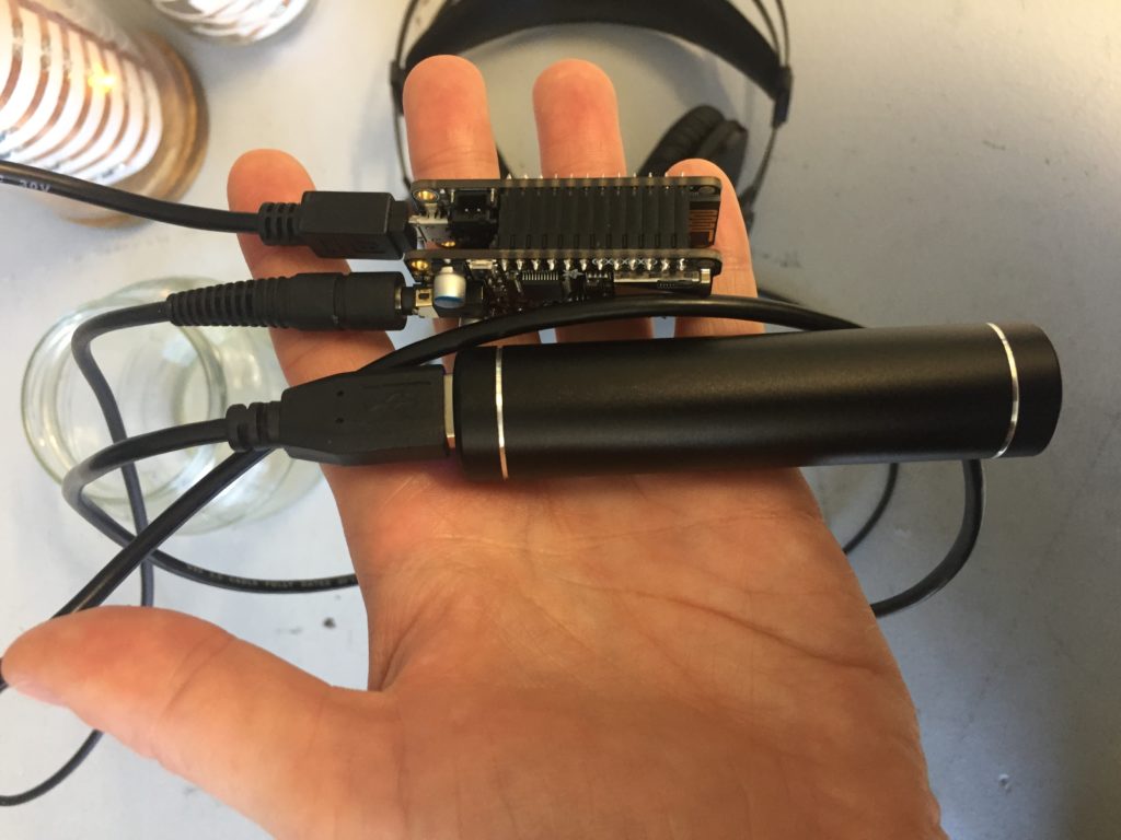
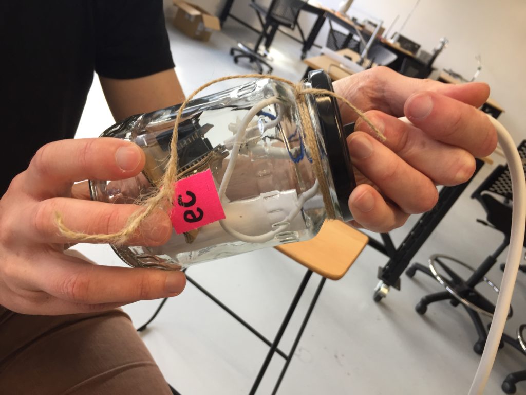
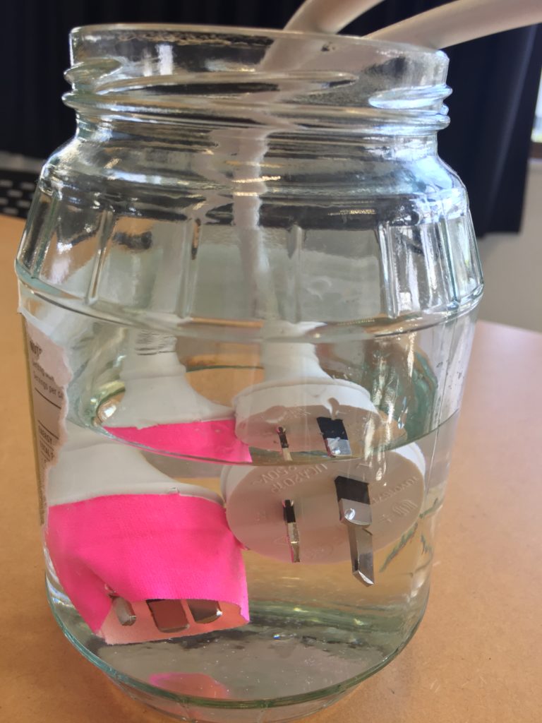
The circuit appears quite fragile, the copper wires can be bent and crushed in the hand which gives it quite a unique aesthetic when handheld. Once transferred into a glass jar, the intricacies of the circuit design fade into the background, and the bright blue LEDs, as well as the battery and the small circuit board, distract from the fragile wires. I programmed the board with a simple test sketch that loops through the three LEDs.

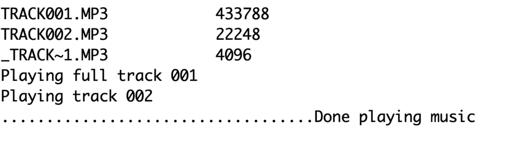
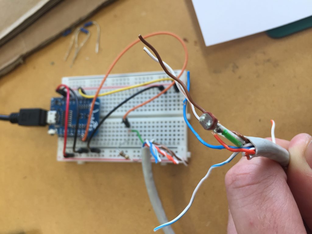
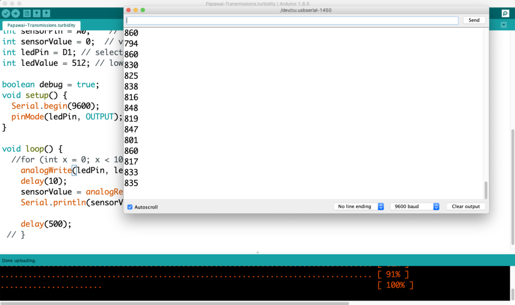
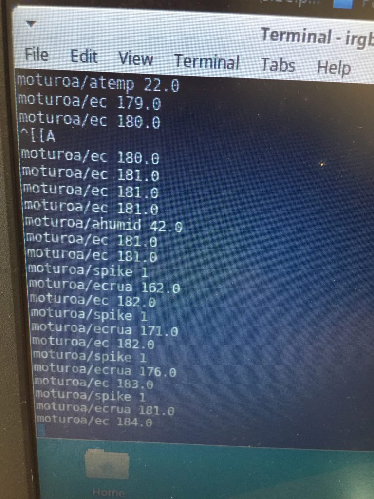
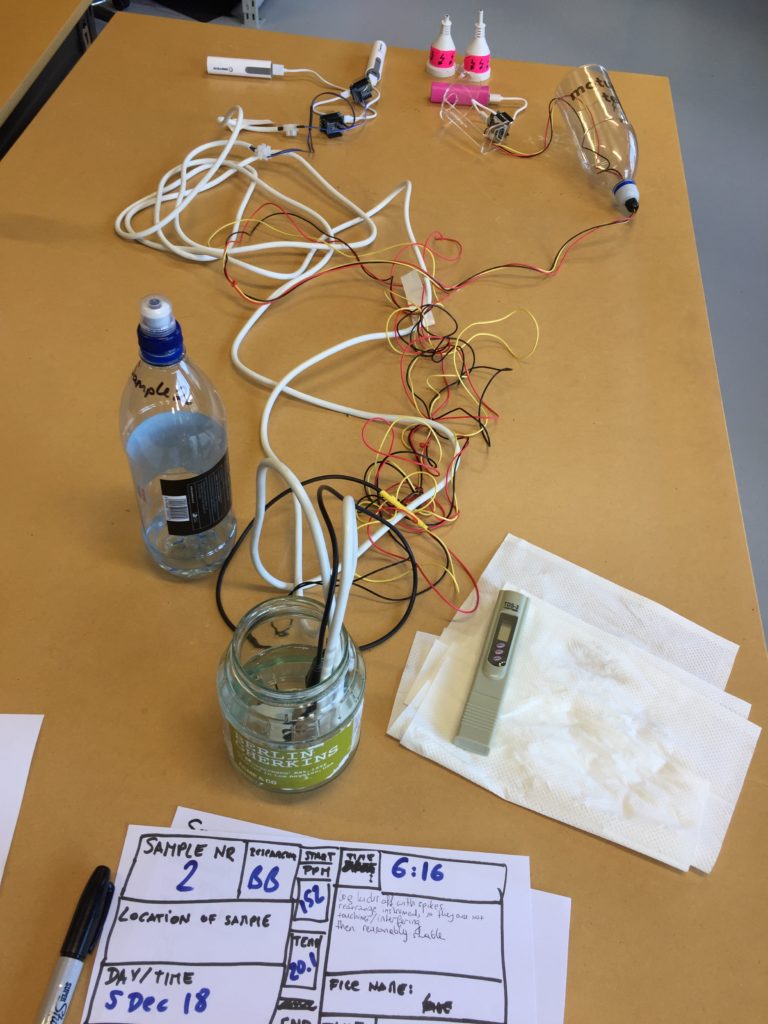
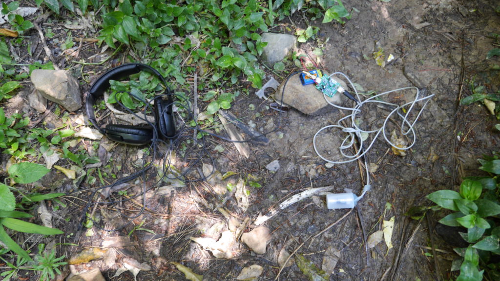
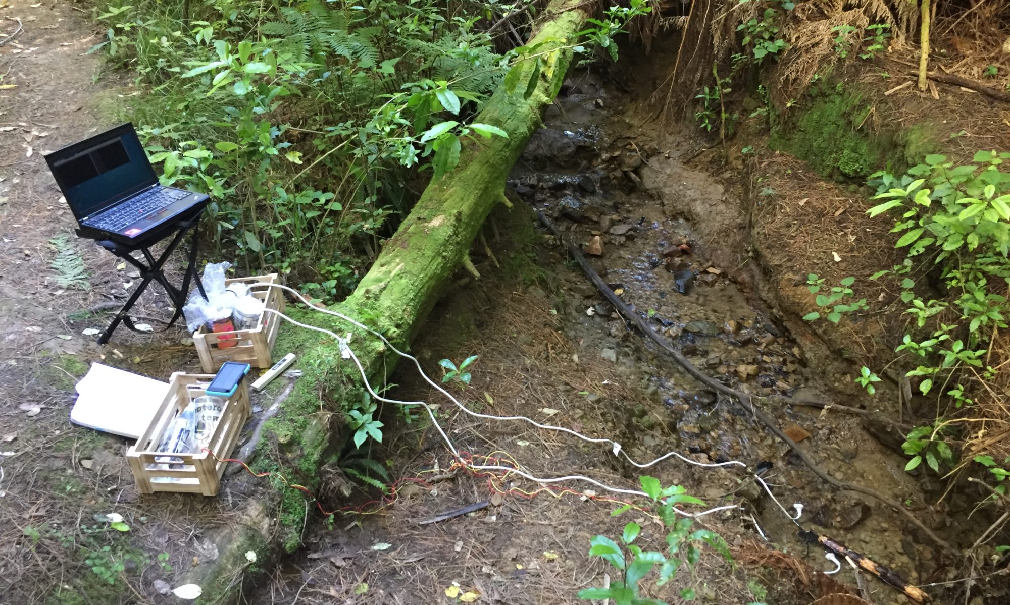
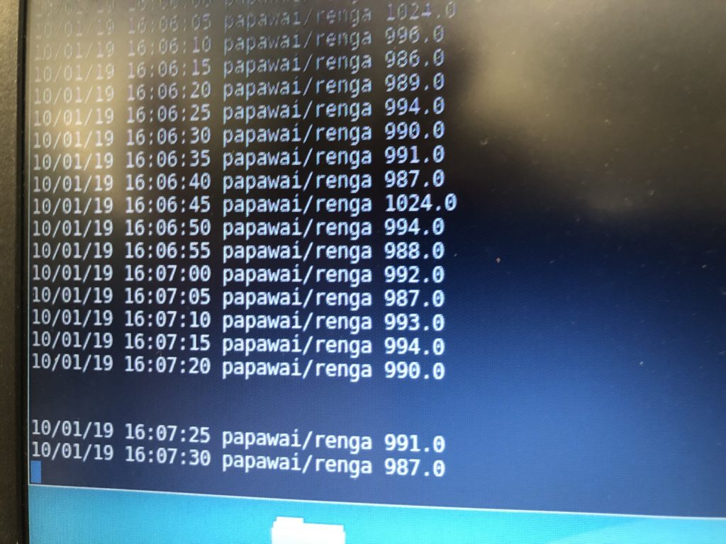
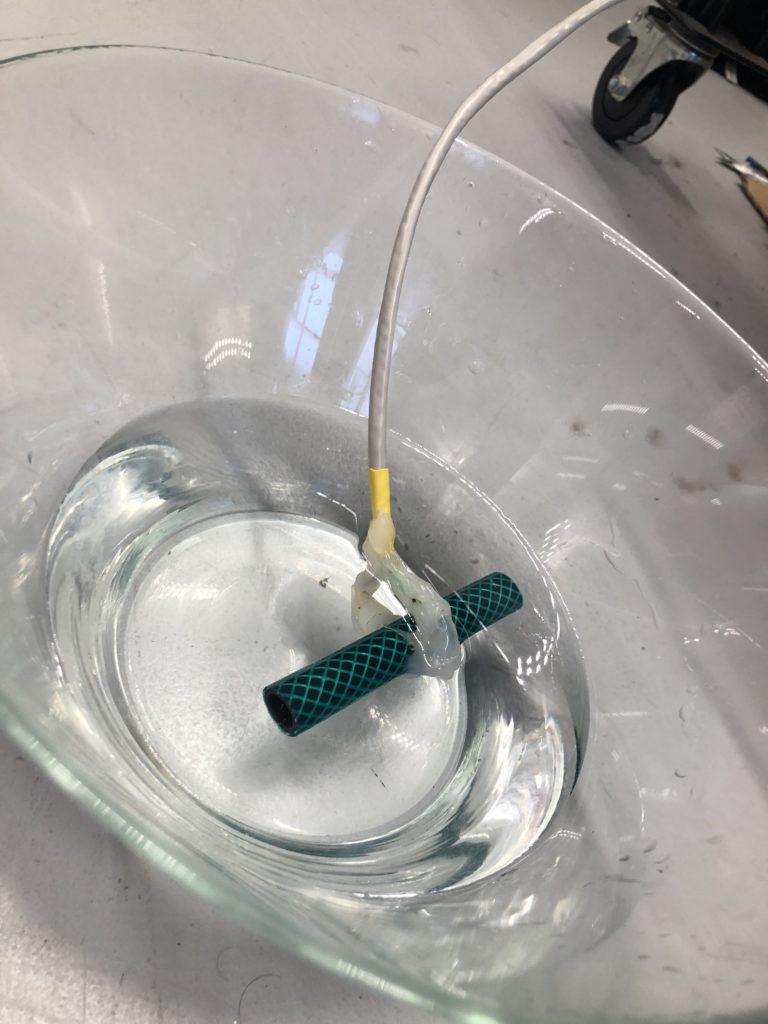
The next step involves connecting this design to the turbidity sensor through my local MQTT network. I submerge my turbidity sensor into a glass bowl filled with water to get more realistic sensor data readings for this test. Unfortunately, the circuit design appears to be tricky to be programmed, and only after a while am I able to successfully de-tangle the wires that must have short-circuited somewhere, causing the code to malfunction and print nonsensical glyphs in the serial monitor when I try to debug my code.

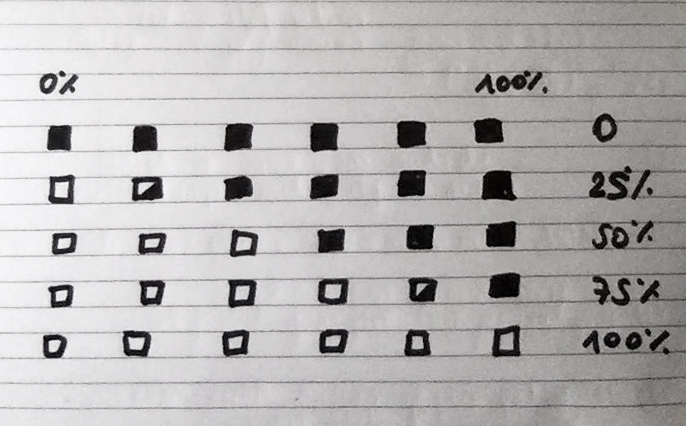
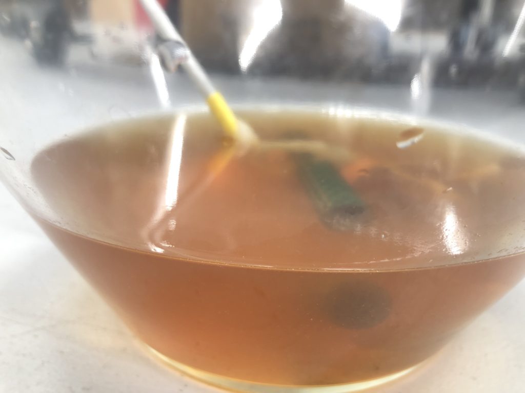
Once my LED node is properly connecting to the WiFi network and correctly receiving the sensor data I map the turbidity to the amount of LEDs being switched on. To achieve a more murky fluid for this test I add a teabag to the water. I notice that the value changes are not as extreme as i would have hoped for and assume that a different resistor, perhaps a trimpot, would help to get more accurate data. Another issue with the sensor data is jumpiness. This could be because the LDR is just not suitable for an accurate measurement, or perhaps the sensor design is not waterproof and hence unreliable. Perhaps the code could be improved by measuring a running average over a couple of miliseconds, instead of measuring the brightness only once sand immediately transmitting this data.

Despite issues with the quality of sensor data, I learned a lot about the feasibility of this circuit design. While the copper wire gives the circuit a unique, messy look that I generally like, it is unsuitable for providing an easily understandable visualization of sensor data. Using only copper rods in combination with 3mm LEDs could work with a refined sketch on how to accurately map the sensor reading to an arrat of LEDs.

Turbidity Output

For this turbidity LED prototype, I wanted to test if I could use a transparent material instead of paper. This would make the microcontroller and the battery more visible and provide more literal transparency in the design.

Planning an designing the circuit

To avoid more plastic usage I recycled an old bottle from the Moturoa installation for this prototype. As a first step, I removed the Moturoa stickers and cleaned it with methylated spirits.

During my initial research I looked for known scales or visual indicators for turbidity but mostly found visual gradients.

My first idea for visualisation was to link the brightness of an LED to the sensor value. For example, if the LED is at full brightness this means the water is clear; if it is of low brightness the visibility of the water is low. An issue with this approach is, that it might be difficult for a viewer to estimate the maximum brightness of a single LED. Hence, a viewer might not be able to extract meaning from the displayed value. LED brightness is generally a hard thing to estimate, especially in bright sunlight.

A solution could be to have a reference LED next to the indicator LED that is always at full brightness as a comparative value. The indicating LED could also be faded on first to a complete maximum brightness and then dimmed to the readout value read by the sensor. This could work, but this method might be too complex and create confusion on how to understand turbidity.

A simpler idea would involve visualising turbidity with an array of LEDs. If water clarity is at 100%, all LEDs are on. At 0% all LEDs are off, at 50% half of the LEDs are on (see sketch above). Using a variable brightness of the rightmost LED could work here to indicate a finer range of turbidity (25% would be one LED on maximum brightness and the neighboring LED at 50%). This idea is simple but does align with the design of previous prototypes. The Wemos D1 mini has nine digital pins in total. I chose to use six LEDs for this prototype because this allows seeing all LEDs from one angle while leaving enough space (around 15mm) in between the 5mm copper tape lines.

Assembly of the copper tape circuit

The plastic insert should fit inside a glass jar and it should be fitting into a variety of jar sizes. I place the six copper trails to the digital pins on the top of the plastic cylinder. I decided to line the bottom of the cylinder with one continuous piece of tape as ground (GND).

For this light probe, I chose blue SMD LEDs, mostly because I haven’t used this colour in any other probes so far. I apply some solder on the copper tapes first before placing the SMD on the circuit with a pair of tweezers. Then I melt one solder to tentatively put the LED in place before finalising the solder points on both sides. As anticipated, plastic and copper tape are not an ideal combination. Too much heat from the soldering iron melts the tape layer of the copper tape and lifts it off the surface (as with paper). The heat additionally shrinks the plastic and eventually deforms the entire surface.

Before adding another LED I test every solder connection immediately by connecting a 3V power supply. This involves checking whether the solder point is good enough and if the polarity of the LED is correct. This batch of LEDs was easier to place on the circuit as they feature a clear polarity mark on the top.

To finalise the circuit I decided to solder copper tape ends together instead of taping them. Using sellotape to bridge copper tape ends has turned out to be a weak connection point in previous prototypes. This turned out to be a problem especially once I needed to bend the paper circuit to fit into the jars. The soldered connections are more stable and reliable. Unfortunately, the additionally applied heat and solder gave the GND copper tape a somewhat messy look.

Connecting the circuit to the micro controller

After placing the finished circuit into a glass, aesthetic details of the copper tapes become less obvious. The bright blue LED becoming the visual focus of the prototype.

The final soldering job involved attaching wires to the circuit that could connect to the WeMos D1 mini microcontroller.
I chose a piece of CAT5 wire and first soldered seven strands (6 digital pins plus 1 GND) to a row of pin headers to be plugged into the microcontroller. Once completed, I soldered them one by one to the copper tape circuit.

The assembly of the electronic components of the prototype are completed now. The next step involves writing code to link the LED brightness to the readout of the turbidity sensor.

Turbidity Sensor III – One more time

The next iteration of the turbidity sensor requires more thorough waterproofing from the beginning. Prototype I started as a simple proof-of-concept of the component combination ( LED, LDR in a garden hose enclosure) and had no consideration of waterproofing. After that, the focus of Prototype II lay on improving the initial design’s lack of water-proofing and adding long cables so it can be eventually tested out in the field.

Part I: Components, cables and heat shrinking tube

For this turbidity sensor design, I used an approximately two-meter-long stranded core CAT-5 cable to connect my white LED and my LDR to my Wemos D1 board.

After assembly, I immediately sealed the components that eventually get submerged into the water with heat shrink tubing (yellow for the LED, green for the LDR).

My first attempt at running the test code with the components through the two-meter-long wire went well. I tested the incoming values roughly by concealing the LDR with my finger.

Part II: Housing the components in the “test tube.”

Similar to the previous prototype, I cut a new 10cm piece off the garden hose and drilled two opposing holes of the size of the components in the centre. To attach the LDR and the LDR I used hot glue only this time. The reasoning behind this is that hot glue has a much shorter drying/hardening time than the All Clear sealant. This allows an efficient applying of layer after layer within a relatively short period. The sealant ideally requires overnight drying which means assembly would span several days instead of hours.

The work with hot glue is messy and requires diligence. Therefor, the purpose of the first layer is to attach the components to the hose and make sure they are facing each other correctly.

After the first layer has been applied I test that the components have not been damaged in the process of hot glueing. The incoming values look good so far, but I am not entirely happy with the design. It is quite hard to apply hot glue around the components evenly. I already spot some small grooves in the glue that could cause some leaks later on.

Part III: Dear hot glue, please protect my components

While applying the next layer of hot glue, I have already made peace with the fact that this probe is going to look very odd. Basically, I am looking at a small dark-green piece of garden hose attached to a long cable with semi-transparent blobs of glue. I also notice that the wire close to the components appears to be under strain caused by the angle the components are attached to the hose. I should have immediately bent the connectors at a right angle to avoid this oddly shaped glue blob altogether.

Despite the aesthetic shortcomings of this turbidity sensor design all components seem to be working, and I am ready to compile a version that sends data wirelessly via the MQTT network so I can safely test the design in an underwater setting, without the need of a laptop attached to any submerged components.

References
donblair. (2015, August 25). Turbidity 001. Retrieved January 18, 2019, from publiclab.org/n/12168
Kelley, C., Krolick, A., Brunner, L., Burklund, A., Kahn, D., Ball, W., & Weber-Shirk, M. (2014). An Affordable Open-Source Turbidimeter. Sensors, 14(4), 7142–7155. https://doi.org/10.3390/s140407142
NIWA. (2008, December 17). Training notes. Retrieved January 28, 2019, from https://www.niwa.co.nz/our-science/freshwater/tools/shmak/manual
/15trainingnotes
Open Water Project. (n.d.). Open Water Project. Retrieved January 28, 2019, from https://github.com/OpenWaterProject

Giving voice to the stream: An audio node part I

Several participants in my design evaluation interviews indicated the interest in having audio as a medium to access the stream sensor data. As a result of this, I looked at options to use the ESP8266 chip in combination with a simple audio interface. I found some research on using the Wemos D1 for sound applications, a previously purchased microcontroller, the Adafruit Feather Huzzah can be expanded with the Music Maker FeatherWing, which adds an audio interface with a headphone jack output which could be used as a standalone version in the field.

Setting up the Adafruit Feather Huzzah

The Feather requires you to install a USB-driver (USB to UART Bridge VCP drivers) to work with your operating system properly. Note: For this install you need to restart your computer.

The Huzzah is part of the ESP8266 board manager, which needs to be added to the Arduino IDE under via Arduino…Preferences…Additional Board Manager URLs…

If step one and two have been successful, the Feather should be ready to be programmed with the Arduino IDE.

Arduino…Tools menu showing correct Board and Port to work with the Feather

Success. The Blink sketch is running smoothly on my Feather.

    Feather Huzzah running the Blink script
Equipment Cost

I have ordered the Feather ordered at an earlier stage of the research project, but decided in the and not to chose it as the chosen as a central component of my project, mainly because of the price point (currently $33.00pp vs Wemos D1 $10.00pp on nicegear).

The Musicmaker shield adds another $36.00 to the sum.

For a complete audio player setup, an SD card (to store the mp3 files) and headphones are required. The MIDI setup does not require the SD card.

Adding the Audio Shield

Once the Musicmaker arrives I need to install some software as described in the guide by lady ada (2018):

  1. Install the library for the Adafruit VS1053 Codec Breakout (lady ada, p.13).
  2. Test the example code feather_player with two mp3 files on the SD card.
  3. Solder the MIDI jumper on the bottom of the board together and test the MIDI example.

So far so good.

Now I need to connect the Feather to my MQTT network and have audio play triggered by a callback.

After some fiddling with the code, I manage to play the test Ocarina scale from the example code when the EC sensor and the water temperature sensor transmit data across the network.

The audio jar stands now among two visual outputs. While it offers a different mode of access to the stream data, it also breaks with the convention of having one-on-one relationships between input and output nodes.

I also need to consider if the jar casing is the best choice for this node, and how an audience would access the data in the field. The node could be a hidden audio jack that participants can plug their headphones into, or headphones can be provided. Alternatively, I could use a small speaker to play the sound output and make the experience accessible to multiple users at the same time.

The opportunities for this extra node need to be tested and evaluated in the field.

References
adafruit. (2019). Adafruit_VS1053_Library [Arduino]. Retrieved from https://github.com/adafruit/Adafruit_VS1053_Library/archive/master.zip
lady ada. (2018, August 22). Adafruit Music Maker FeatherWing. Adafruit Industries. Retrieved from https://learn.adafruit.com/adafruit-music-maker-featherwing

A stream wellbeing LED jar: Water Temperature Visualization: Part I

My DIY water sensor nodes need field-compatible outputs so that visitors can easily access and understand the sensor data of the IoT network in real-time. The design for the temperature visualisation is based on the concept of the previous paper circuit for the EC probe, because research participants generally gave the design with cardboard, copper tape and white LEDs positive feedback. For the water temperature jar, however, I am using coloured LEDs, as suggested by one participant. In my development notes below, you can learn how I designed and assembled the device, and how the SHMAK manual (NIWA, 2008) helped to make the visual output meaningful. The idea for using cardboard and copper tape for these prototypes is inspired by the work by Jie Qi (2012) and the High-Low Tech Group at MIT Media Lab (2012). 

Development Notes

Similar to the previous LED prototype I use a 12cm high sheet of white card paper as a base for my copper tape trails. During an evaluation discussion on the EC jar design, participant 18 suggested the use of coloured LEDs for future iterations. I am attempting to implement this suggestion in the design for the jar that visualises the data coming from the water temperature sensor (DS18B20).

Evaluating the EC jar design with research participant in the lab (Jan 2019)

Visualising stream wellbeing

During the ideation phase, I focused on a suitable way to connect coloured lights meaningfully to the water temperature readouts. Hence, instead of opting for a traditional water temperature colour scale for blue (cold) and red (warm) I departed from the perspective of the stream, and what effect water temperature has on the more-than-human wellbeing of the stream.

Water temperature

Water temperature

Stream temperature is important because every species has a preferred temperature range. The range varies considerably from species to species. Sometimes, a temperature change is important, for example, as a trigger for egg hatching in some mayflies. Many organisms are unable to survive in temperatures above about 30 °C (except for some adapted to life in hot springs). At the other end of the scale, temperatures below freezing point constitute a very harsh environment because of the effects of ice.

A single temperature measurement is not particularly informative, but a series over time will provide a rough picture of the temperature regime in a stream. The longer the series and the closer together the measurements, the more informative the series will be.

Temperature depends largely on time of year and weather conditions. Stream type also plays a part. For example, lowland streams tend to experience quite stable temperatures (i.e., closely following average air temperatures). Shading along streams reduces the occurrence of extremely high water temperatures.

Water temperature fluctuates on a daily basis and for this reason it is suggested that measurements are always conducted at the same time of day.

Less than 5
Rating: fair
Score: 5

Less than 5°C

Values below 5 ºC are low and indicative of winter conditions in southern regions. Invertebrate and periphyton growth would be slow in such waters. Some species may be excluded.

5 to 9.9
Rating: good
Score: 8

5 to 9.9°C

Values of 5 to 10°C are moderate to low and indicative of winter conditions. Most invertebrates and periphyton can survive well in these temperatures.

10 to 14.9
Rating: excellent
Score: 10

10 to 14.9 °C

Values of 10 to 15°C are very suitable for most invertebrates and periphyton.

15 to 19.9
Rating: good
Score: 5

15 to 19.9°C

Temperatures of 15 to 20°C will start to be stressful for some invertebrates (e.g., stoneflies).

20 to 24.9
Rating: fair
Score: 5

20 to 24.9 °C

Temperatures of 20 to 25°C are moderately high. Some invertebrates, such as some mayflies, stoneflies, and some fish, such as trout, are unlikely to survive such conditions for prolonged periods (e.g., several weeks).

25 to 29.9
Rating: poor
Score: 0

25 to 29.9 °C

Temperatures between 25 and 30°C are likely to be stressful to fish, stoneflies, mayflies and some caddis flies. Such high temperatures may be a result of lack of shading and very sluggish flows.

30°C or more
Rating: poor
Score: -5

30 °C or more

Temperatures over 30°C are likely to be very stressful to most stream life and result in their death. Again, such high temperatures may be a result of lack of shading and very sluggish flows. However, stream temperatures will rarely get to these levels.

Table 1: Habitat indicators of stream health. From NIWA (National Institute of Water and Atmospheric Research), 2008.

The table contains seven water temperature bands rated from poor to good. I opt to use one LED for each band, representing the ratings (poor, fair, good, excellent) with colour. I choose red, yellow and green LEDs to indicate the stream health rating:

Red Poor
Yellow Fair
Green Good
Green x2 Excellent

Copper tape circuit design and assembly

To accelerate the development, I aim to build simple straight copper trails first as a proof of concept instead of spending time on developing a unique visual aesthetic for the circuit design without knowing whether the general concept works. I use the same circuit design as for the LED jar, but I need to recalculate the spacing for this version to fit eight rows of copper tape on the paper.

The Wemos D1 has seven digital outputs which makes it suitable for addressing seven LEDs individually. With the 8th digital output unused there is an opportunity for of adding a white LED on top later crossing all other outputs with sellotape, that could indicate the status of the network, similar to the EC jar.

The biggest challenge when making circuits with copper tape is the needs careful treatment and patience to make sure connections don’t break.

I use a craft knife to make precise cuts where the LEDs will be soldered in later.

I align the LEDs on the page so that the output can be seen best from one single perspective, that should later face towards an accessible area by the stream.

After all the LEDs are soldered into the circuit I test the quality of my solder points with a voltmeter.

Then I manually apply the forward voltage of each LED separately to test whether the connections work up until the edge of my circuit, where I will later add the connections to the microcontroller.

Challenges, reflections and learning outcomes

When working with SMD LEDs, I encountered the following issues:

  1. The LEDs are tiny and their polarity is barely visible from the top.  Sometimes LEDs move during soldering or don’t connect properly. I need to make sure I don’t accidentally move or flip them when working on the circuit touching the circuit with my hands or the tip of my soldering iron.
  2. The LEDs that I am using have a clear lens. I need to be careful to not mix up LEDs of different colours. The only way to know their colour is to power them on, which is tedious when dealing with the SMD form factor.
  3. Components close to each other don’t work well with copper tape. There need to be at least some centimetres of tape between two components.

In the sketch above you can see that my reference paper for the LEDs has moved in the process of adding LEDs which resulted in me picking the wrong LEDs for the first two rows. After removing the wrongly coloured LED I also realise that two green LEDs in series will not work for the “excellent” category as that would require a voltage of 2*2.2V which the microcontroller cannot supply. After making too many errors, I decided that I call it a day after testing that all the other LEDs work and will continue lab development after a healthy amount of sleep.


References

High-Low Tech Group, MIT Media Lab. (2012, August 21). Paper circuits. Retrieved February 27, 2019, from http://highlowtech.org/?p=2505
 
NIWA. (2008, December 17). Habitat indicators of stream health. Retrieved February 27, 2019, from https://www.niwa.co.nz/our-science/freshwater/tools/shmak/manual/9habitat
 
Qi, J. (2012). The Fine Art of Electronics: Paper-based Circuits for Creative Expression (Master of Science in Media Arts and Sciences). Massachusetts Institute of Technology, Massachusetts, NE. Retrieved from http://web.mit.edu/~jieqi/Public/Jie_Qi_MS_thesis.pdf

Turbidity Sensor II – Improved design with material issues

With this revised prototype I aimed to create a better, more stable design by inserting the LED and the photocell through holes into the hose while improving the sealing of electrical components from the beginning. I also wanted to use a cable with the actual length for use in the field and chose an approximately 2m long stranded core CAT-5 cable.

First I soldered the photocell to the green pair of cables and tested it with the code from yesterday.

I drilled 5mm hole into the hose to fit the LDR neatly.

The 3mm LED requires a 3mm hole respectively. I drilled the 3mm through the 5mm hole to make sure the holes are nicely aligned.

Reconnecting the wires with the breadboard from the previous prototype I ended up swapping the resistor to a 10k one which gave me more consistent readings when the LED was on half brightness.


For the sealing, I purchased the All Clear sealant that I have previously used for waterproofing my hydrophone. As opposed to hot glue, this material stays flexible when dried out and doesn’t run the risk of getting brittle.

Unfortunately one of the LED solder points was not well done, and I only discovered it after having added the sealant. With the cable disconnected, this prototype is unusable in the field, but the process of building it helped me understand possible avenues for improvement:

The design with the components stuck through tight-fitting holes is cleaner but needs to be revised with waterproofing in mind.

Solder points need to be stress tested and – if necessary re-done – before adding sealant.

Cables need to be fixed into place before adding sealant. Sealing might need to be re-done in the 3D workshop with proper ventilation and safety gear as this might require the use of turpentine.

Sealant might need to be changed as it might not be ideal in combination with cables/electronics.


Component List:

Hardware:

  • Computer with USB interface
  • Wemos D1 mini (know known as LOLIN
  • 1 LDR
  • 1 10k Resistor
  • 1 3mm white LED
  • Drill with 3mm and 5mm bits
  • All Clear Sealant

Software

Lab EC-sensor tests

Before using more EC probes in the field and gathering data from different parts of the stream I tested them in a controlled environment in the lab.

Experiment 1: 

The two versions tested use the same materials, same length of chord and same 560 Ohm resistor. The first test involved a jar filled with tap water, immersing both sensors in the jar and monitoring the data via mosquitto_sub.

Jar filled with tap water for testing two DIY EC probes

Note: The pink tape wrapped around one probe was an attempt to avoid the probe mistaken with a power plug on the lab table, which poses a severe hazard. The probes are stored away safely when unattended to ensure health and safety.  This version of the probe uses the Live (L) and neutral (N) prong of the plug. To improve the safety of the probe the live (L) prong should be removed and Neutral (N) and Ground (⏚) should be used for measuring the electric conductivity. 

The terminal output shows the EC probes publishing the measured values under the topics motorola/ec and moturoa/ecrua. While the test recording was done, the DHT11 sensor was also active in the lab, publishing air temperature (moturoa/atemp) and air humidity (moturoa/ahumid). Output showing values returned by two EC probes (moturoa/ec and moturoa/ecrua) and DHT11 sensor showing air temperature (moturoa/atemp) and air humidity (moturoa/ahumid)

This first test showed a deviation of around 10 between both probes, behaving relatively consistent. The next test would require measurements in the stream to see whether the probes return coherent readings from flowing  water.

Experiment 2:

Due to bad weather and high winds it was too dangerous to conduct testing in the field. However, to get a better idea of the consistency between the two probes I went to an easily accessible part of the stream outside of the forested area and collected two samples of stream water. 

Back in the lab I pour the first sample into a clean jar that is big enough to contain all three sensors. I prepared a paper sheet for keeping experiment notes, starting with date/time, location of sample taken, last weather and readings from the TDS meter at the beginning and end of the test.

  1. I boot the Raspberry Pi (the Pi acts as Wi-Fi Access POint hosting the Moturoa_Transmissions network and acts as the MQTT-broker).
  2. Connect laptop to Moturoa_Transmissions and start log with timestamp
    mosquitto_sub -v -h 192.168.42.1 -p 1883 -t '#' | xargs -d$'\n' -L1 sh -c 'date "+%D %T $0"' > data.log
  3. Immerse probes into water sample and activate by connecting the Wemos D1 micro controllers to power supplies (USB batteries).

The raw data of both test results can be found on the development repository.

Building a low-cost hydrophone

For this research I want to explore what kind of DIY electronics can amplify the voice of the forgotten streams in Poneke/Wellington, New Zealand. As a first device I want to build a hydrophone that can be used during fieldwork to record underwater sounds.

Hydrophones used in scientific research, for acoustic monitoring, such as for tracking marine animals, are relatively expensive and even DIY solutions feature costly elements (see for example Dawson, 2012). In low-cost DIY solutions old audio components, such as headphones or radios are re-used (e.g. digifishmusic, 2008) and made waterproof with silicone or hot glue.

I decided to combine building a hydrophone based on two instructions. Both are based on using an electret microphone element as the primary component. In the instructions of Decker (2013) the element is enclosed in an empty film canister filled with mineral oil as a medium to optimize the hyrdophone. I chose this design for the first version following a suggestion on the Wellington Sonic Arts Facebook. The instructions by the University of Waikato (2011) feature a component list that is available in New Zealand.

components used for first hydrophone prototype

Building the first version of the hydrophone took less than a day and involved researching the best possible option to be done within one day, sketching a schematic alongside a shopping list of necessary parts, planning the quickest route around town to buy all necessary parts and then 2 hours of soldering and assembling plus some extra time for testing and troubleshooting and documenting along the way.

detail of the electret microphone in the film canister

detail of the preamp (see similar component here)

hydrophone without casing next to Papwai Stream

I built the hydrophone as described in Decker (2013) but used a 3.5mm mono headphone jack at the end of the 3 meter long cable. I also soldered 3.5mm sockets to the pre-amp for in- and outputs to keep the device as modular as possible. For testing the hyrdrophone I used a pair of headphones, but I will be looking into options for adding a speaker. Currently, the pre-amp turns on and off by connecting and deconnecting the battery, which is cumbersome, so adding a switch would be a good improvement overall to be added to a (preferably waterproof) enclosure.

Dawson, S. (2012, January 20). Building the “CETOS” directional hydrophone. Retrieved from http://whaledolphintrust.org.nz/wp-content/uploads/Building-Directional-HPs.pdf

Decker, F. C. (2013, June). Underwater sound detection using sea perch through construction and operation of hydrophone. Retrieved from https://seaperch.byu.edu/wp-content/uploads/2013/06/Final.pdf

digifishmusic. (2008, January). How to make a Hydrophone (stereo!). freesound. Retrieved from http://www.freesound.org/forum/production-techniques-music-gear-tips-and-tricks/2631/?page=1#post13253

The University of Waikato, New Zealand. (2011, May 10). Make and Use a Hydrophone. Retrieved October 17, 2016, from http://sciencelearn.org.nz/content/download/20964/411858/version/7/file/Make+and+use+a+hydrophone.doc